Field Oriented Control (FOC)

Field Oriented Control is often considered a dark art filled with diagrams, math, and proofs by intimidation.
Often people will show a diagram like this,
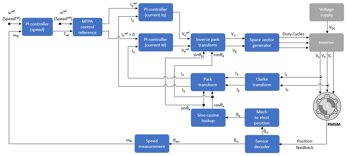
and pretend like it's self explanatory.
Not true!
However, once you get an understanding of what the different pieces are and what they are trying to do, you'll realize that it can be quite intuitive.
Let's dive in.
1. How does a motor work?
Let's start with the humble goal of understanding how a motor works.
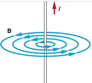
When you run a current through a wire, you get a magnetic field around the wire.
If I put a permanent magnet like a compass next to the wire, the magnetic field of the compass interacts with the magnetic field around the wire which causes the compass to be deflected.
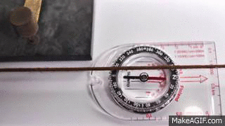
This is a result of the north and south poles of each field being attracted to each other and trying to align.
A motor works in the same way.
Inside of the motor there are both permanent magnets and wires. When you run a current through the wires inside the motor, the magnetic field of the wire interacts with the magnetic field of the permanent magnets - just like the compass and wire we talked about before.
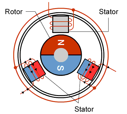
1.1 Motor Terminology
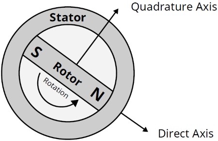
There are two main parts of a motor: a rotor and a stator.
The rotor is free to rotate and the stator is stationary.
The permanent magnets are attached to the rotor and the wire is wrapped around specific parts of the stator.
Now if I start to run current through the wire, I get a magnetic field that starts to interact with the magnetic field of the permanent magnets. Since the permanent magnets on the rotor are free to rotate, the rotor will rotate to try to align its magnetic field with the one created by the wire.
And so, we get a rotation. Success!
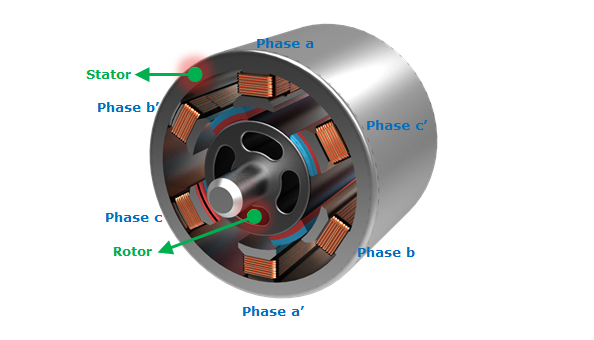
This type of motor is called a Brushless DC motor (BLDC) and a variant of it called a Permanent Magnet Synchronous Motor (PMSM) is what we'll be focusing on in this post.
Depending on the motor design, there may also be sensors like hall-effect sensors or encoders inside the motor that provide position data. We'll touch on these later.
2. How to spin efficiently
Okay, so we know that putting current through the motor wires makes the motor spin, but how do we know when to stop running current through one set of wires and run it through a different set of wires so that the motor can keep spinning?
If you take a step back for a second and think about what we want to do, the ideal direction for the force that we want to apply is for it to be tangential to the rotor like this:
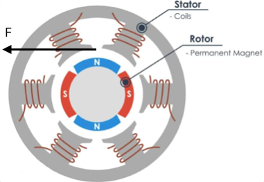
This maximizes the torque applied to the rotor and makes it so that all of the force (and energy!) that we use goes to achieving our goal of rotating the rotor.
So if we can get the magnetic fields created by the currents in the wire to interact with the permanent magnets in such a way that the magnetic force is applied tangentially to the rotor, then we know we are driving the motor in an efficient way.
But how do we that?
This will come down to how the wire inside the motor is wound since the path that the wire is taking will determine the path of the magnetic field when we run current through it.
There are two ways in which motors are typically wound: concentrated and distributed.
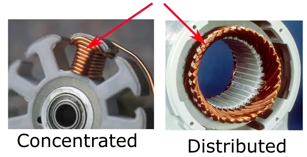
BLDC motors tend to have concentrated windings whereas PMSM motors tend to have distributed windings.
Because of the interaction of these distributed windings with the permanent magnets in a PMSM motor, the optimal way of driving the motor is to use a 3 phase sinusoidal waveform like this:
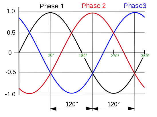
Thus, FOC's job is to create this smooth 3 phase current through the 3 windings in the motor.
3. How does FOC do that?
The core idea of FOC is to continuously adjust the stator currents so that the magnetic field they produce is always 90° orthogonal to the rotor’s field.
If you only take one thing away from reading this, let it be that previous statement.
The goal of all of the fancy math, sensors, and PI controllers is to make sure that statement holds as close to true as possible at all times during the motor's operation.
FOC does this by converting to a frame of reference where it is easy to control the stator current magnetic field which produces torque.
Once you have an "easy" way of controlling the torque, you can get the motor to perform arbitrary commands.
But what do I mean by "easy"?
Specifically, "easy" as we will see in FOC means that we command a specific current (which produces torque) and we are able to track it as a time-invariant DC signal. This allows us to use something as simple as PID control to control the motor, even though the phase currents themselves are actually time-varying sinusoidal signals. Therefore, instead of having to control time-varying sinusoidal signals, we can control time-invariant DC signals.
That last point is worth repeating.
FOC allows us to turn the difficult problem of controlling 3 time-varying sinusoidal signals into an "easy" one of controlling two time-invariant DC signals.
To see more clearly how FOC does all of this, we have to dig a little deeper.
4. Digging deeper
In this section we're going to get into the specifics of FOC along with all the math, etc.
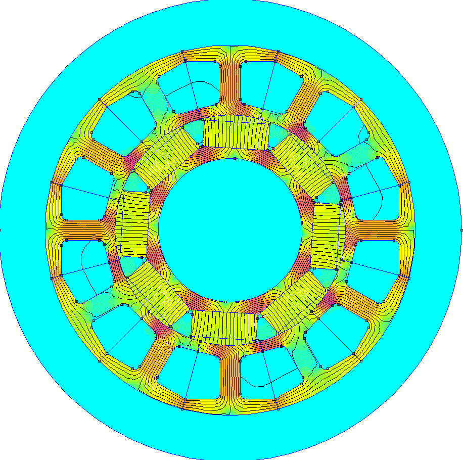
Our goal is to get a smoothly rotating magnetic field like this to be created by only changing the currents flowing though the 3 windings.
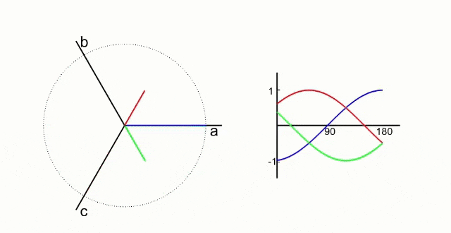
The green, red, and dark blue lines are vectors representing the magnetic field created by the current flowing through each winding and the cyan line is the combined magnetic field resulting from the interaction of the 3 magnetic fields.
The important thing to see here is that the cyan vector is smoothly rotating around the circle which results in the magnetic field from the stator currents being applied tangentially to the permanent magnets like we want.
It might take a couple of reads for everything in this section to click, but just keep in mind the concepts from the previous section if you get stuck.
4.1 Motor Schematic
A PMSM motor can be modeled electrically as follows,

This is our initial frame of reference where we can measure stator currents and output stator voltages.
If we apply Kirchoff's current law at the point in the middle of where the 3 windings meet, we get the following equation,
This equation is very important.
What this is saying is that even though we have 3 axes (one for each winding that the current can flow through), we only have 2 degrees of freedom.
So why is this important?
4.2 Clarke, Park, and friends
What we are looking for is a way to represent the magnetic field created by the 3 phase currents using a reference frame with two axes: one that is aligned with the magnetic field of the rotor and another that is perpendicular to the first axis.
The second axis would give us the direction to apply a force in order to maximize the torque to spin the motor.
This would allow us to control the torque being applied to the rotor by changing the 3 phase currents.
Something like this would be ideal:
This is what the Clarke and Park transforms allow us to do.
4.2.1 Clarke Transform
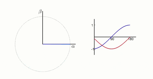
The Clarke transform maps the 3 stator current axes into 2 axes called and .
The only reason we can map 3 axes into 2 axes without losing any information is because we only have 2 degrees of freedom (not 3) like we saw in the last section from Kirchoff's law.
Also notice that there isn't anything special about the current here. We can also do the same thing with the phase voltages to get,
These equations might seem mysterious at first, but look a bit closer: the axis is aligned with and axes and are projected into a single axis that is perpendicular to (and thus also perpendicular to ).
If you're familiar with linear algebra, this is doing what's called a change of basis. In fact, in matrix form the current can be expressed like this,
Geometrically, this gets us to here.
That's a good start, but this would still require us to control two sinusoidal waves when doing control.
Can we make the control easier with another change of reference frame?
4.2.2 Park Transform
It turns out that we can.
If you think about it, the sinusoidal waves are coming from the fact that in the current frame of reference, the current vector is rotating.
But what if we make the entire frame of reference rotate?
If we can transform the alpha-beta frame into a frame of reference that rotates, then from this new frame of reference, the current is not rotating. In fact, it would look stationary.
What we want is something like this:
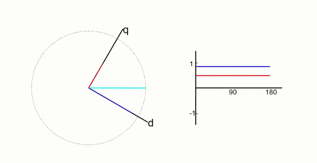
This is what the Park transform gives us.
By doing another change of basis, we can make the signals that we want to control look as though they are DC signals.
This is great, because controlling DC signals is straightforward.
In this frame of reference, is called the direct axis current which represents how much current is aligned with the rotor’s field (producing no torque, just magnetizing or de-magnetizing by modifying the magnetic flux). is the quadrature axis current and is perpendicular to the rotor’s magnetic field (producing torque).
In our case, we want all torque and no extra magnetization, so we want and we want to be whatever is needed for the desired torque.
Stop for a second and think about this. What we've done here is pretty incredible. We now are able to command the exact torque and flux we want from the motor in a non-coupled time invariant way using only the stator currents.
As we'll see later, this allows us to control the flux and torque like DC quantities using classical PI regulators.
This is the whole reason for using Field Oriented Control: AC phase currents get controlled via DC targets in the rotating d–q frame.
4.2.3 Inverse Transforms
An important feature of the Clarke and Park transforms is that they can be inverted. Remember, we didn't lose any information so we should be able to "undo" the transformation.
Rearranging the Park transformation above we can solve for the Inverse Park Transform to get,
Similarly for the inverse Clarke transform we get,
However in practice, we use the inverse Clarke and inverse Park transforms to get phase voltages, not phase currents. This is because we can't directly command a current, but we can directly command a voltage by turning the FETs on the inverter on and off using PWM.
Thus in practice you'll see this version of the inverse Park transform,
and this version of the inverse Clarke transform,
Now that we have a way to turn our stator currents into DC signals (and back), it's time for controls.
4.3 Speed loop and Current loop
There are three PI loops in most FOC implementations: the (outer) speed loop and two (inner) current loops.
The outer speed loop takes the commanded speed that we want the motor to spin at, compares it with the measured speed, and uses a PI controller to output a commanded torque (in the form of a current since current is proportional to torque).
The inner current loop takes the output current of the speed controller, compares it with the measured current that we get from transforming the phase currents using the Clarke and Park transforms into the - axis, runs this through a PI controller, and hands this off to the inverse Park transform to eventually be fed to the inverter FETs after Space Vector Modulation.
On the other hand, for our use case, the inner current loop will always be driven to zero. This is because any current on the axis would waste energy since it would not contribute to maximizing the torque generated by the stator current magnetic field.
4.4 Position and Speed
I'm going to keep this section short since the way you get a position and speed estimate of the rotor is heavily motor dependent.
Broadly, there are two ways you can get estimates for speed and position: sensored and unsensored.
In the unsensored case, you'll run the voltage and current values of each phase in the - frame into either a sliding mode observer or a Kalman filter of some kind. Sliding mode observers are more common since they tend to be easier to tune.
In the sensored case, you'll use either a hall effect sensor or an encoder to get the position of the motor. Hall effect sensors don't have as high of resolution as an encoder but they are good enough at low speeds where the back-emf and currents are hard to discern from noise.
In either case, you can take the delta of subsequent position estimates to get an estimate for speed.
Regardless of how you go about getting your estimates for speed and position, speed gets fed to the speed controller and position gets fed to the Park transform.
4.5 PWM Generation
Great, the inverse Park transform gave us the stator‑voltage vector we want – but how do we turn that into real gate signals for the three half‑bridges?
There are two ways of doing this:
- using the inverse Clarke Transform and normalising each per‑phase reference to the DC‑bus voltage to get a duty‑cycle between 0 and 1
- Space vector pulse width modulation
Both of these achieve the same thing so I'll only discuss 1.
4.5.1 Inverse Clarke and Normalizing
This is the most straightforward approach.
First let's use the inverse Clarke transform to transform the desired voltage vectors back to the frame,
Now let's normalize those to our PWMs,
These are the duty cycles that we use to command our FETs.
Note that we are assuming that the duty ranges from 0 to 1 and that the inverter produces a phase voltage ranging from to .
In practice, I stick with this approach for generating the PWMs over SVPWM because of its simplicity.
5. Understanding the block diagram
Now we can take a look at a standard FOC diagram and try to make sense of it.
Everything that's here we've discussed at a high level, so let's break it down piece by piece and walk through one iteration of the FOC controller to make things sink in.
First of all, on the right hand side in gray we have the path from the voltage supply to the inverter to the motor. Without this path, we wouldn't have a way of getting current through the inverter and into the motor. Simple enough, moving on.
Next we have the position feedback from the motor. Like we discussed before, this can come from either sensors inside the motor or something like a sliding mode observer (not shown in the diagram). These allow us to get an estimate of the angular speed to give to the speed controller as well as the angular position to give to the Park and inverse Park transforms.
The Clarke transform takes the phase current measurements, turns them into the - frame, and passes them to the Park transform. The Park transform takes these, converts them into the - frame
Next we have the outer speed loop. This takes the motor's measured speed as well as the commanded speed and runs it through a PI controller. The difference between the measured speed and the commanded speed is what is considered the error and is what we are trying to drive to zero. The output of this controller is run through the MTPA to check to make sure that the current being commanded is below the maximum limit and the result is passed into the inner current control loop that is controlling .
Like we mentioned earlier, the first current loop controller drives the current to zero in order to not waste any energy driving current in a direction that does not produce torque.
The other current loop takes the output of the MTPA (or speed loop) as well as the measured current, runs it through a PI controller, and hands it off to the inverse Park transform.
The inverse Park transform takes measured currents as well as the outputs of the current loop controllers, transforms them into the - frame, and hands that off to the Space Vector generator which converts those into PWM values that are used to command the FETs.
5.1 Practical Considerations
FOC requires relatively powerful microcontrollers in practice due to how fast the PI loops need to be as well as the math that they are performing.
The current loops tend to run around 20KHz in practice while the speed loop tends to run anywhere from 100Hz to 2000Hz.
The current loop needs to be fast enough that to the speed controller the current looks "stable". Running the current loop around 10 times faster is a heuristic often used in practice since it produces good enough results.
It's also important to note that even if you tried to run the speed loop faster, it won't make that much of a difference since the current will always be able to change much faster than speed can be modified since getting a motor to spin faster takes a lot longer than getting current to increase.
6. Closing
Hopefully this makes FOC a bit less mysterious. The concepts themselves aren't too crazy once you see what the different pieces are and how they fit together.
And remember that FOC is not going anywhere any time soon so if it takes you a couple of passes to understand everything, no big deal.
Just keep the big picture in mind and everything will slowly become more clear.